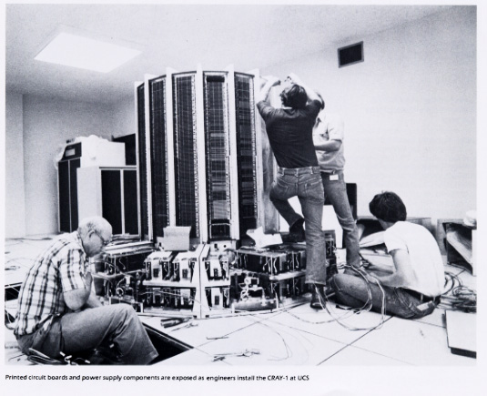
 Cray 1 Install at UCS Photo
This Cray supercomputer Faq is split into sections, Part 1 describes Cray supercomputer families, Part 2 is titled "Tales from the crypto and other bar stories", part 3 is "FAQ kind of items", part 4 is titled "Buying a previously owned machine" and part 5 is "Cray machine specifications". Corrections, contributions and replacement paragraphs to CrayFaq0220@SpikyNorman.net Please see copyright and other notes at the end of each document. Note: Part 3 is the only part posted to newsgroups, the latest version of this and the rest of the documents can be located in http format just down from:
Line art not to scale.
1972    Very Approx.  Time line    1996           (dates not to scale)

                **T3d* --> T3e --> T3e/1200   = MPP
                *     *
C1 -> XMP --> YMP --> C90 ----> T90           = PVP
        \       \      \
      C2 \       \      -> C90M               = Large memory
       . XMS --> ELs ---> J90 -> J90se -> SV1 = Air cooled Vector supermini
         .       APP --> SMP ---> CS6400      = Sparc Superserver
          ....... C3 --> C4                   = Cray Computer corp.

 Key :
 --> Direct architectural descendant
 \   Similar architecture but different technology
 ... Family resemblance
 *   Hosted by
Computers that proudly carried the Cray name can be divided into groups of related architectural families. The first incarnation was the Cray-1, designed and built by Cray Research founder Seymour Cray. This machine incorporated a number of novel architectural concepts that became the foundation for the line of Vector super computers which made Cray Research (1978..1995) legendary in the scientific and technical computing market.
The Cray-1 evolved through a number of, often one-of-a-kind, sub-variants before being replaced by the evolutionary XMP and substantially different Cray-2. This split between the XMP and Cray-2 marked the first divide in the Cray architectural line that together came to define and dominate the super computing market for the best part of 20 years.
The line of machines designated C1, C2, C3 and C4 were the particular developments of Seymour Cray, who split on friendly financial terms from Cray Research in 1989, to progress the Cray 3 project and found Cray Computer Corporation (1989..1992).
In parallel to this, the main body of Cray Research evolved and developed the original Cray-1 concept through four technological generations that culminated in the 32 CPU T90. Along with this a line of compatible mini super computers, an enterprise class version of a scaled-up SMP Sparc architecture and a line of Massively parallel machines were developed and brought to market.
Cray machines were never cheap to buy or own but provided demanding customers with the most powerful computers of the time. Used by a select group of research labs and the top flight of industry, they defined the very nature of supercomputing in the 1980s and 1990s.
This partly compiled from the various SEC 10-K docuemnts and www.top500.org
                                                 CPU Clock
                                    Number of    Cycle time       Memory
System Series       Architecture       CPU's      (in nsecs)    (in megawords)
- -------------     ------------    ---------    ----------    --------------
 CRAY 1                  PVP        1 to 2         12.5         1 to 4
 CRAY 2                  PVP        1 to 4          4.1        64 to 4096
 CRAY 3                  PVP        1 to 16         2.11       64 to 4096

 CRAY X-MP               PVP        1 to 4          8.5         8 to 16
 CRAY Y-MP               PVP        1 to 8          6.0        32 to 4096 *
 CRAY C90                PVP        1 to 16         4.2        64 to 1024
 CRAY T90                PVP        1 to 32         2.2        64 to 1024

 CS6400                  SMP        4 to 64        11.8        32 to 2048

 CRAY Y-MP EL            PVP        2 to 8         30.0        32 to 512
 CRAY J90                PVP        4 to 32        10.0        32 to 1024

 CRAY T3D                MPP        32 to 2048      6.7         8 per CPU
 CRAY T3E                MPP        16 to 2048      3.3         8 to 64 per CPU

 * The Y-MP comes with a 128 Mword SSD as a standard feature.
It is easy to describe the power of these super computers in terms of CPU MHzs and Mflops but the numbers fail to quantify the real difference between Cray computers and the other available machines of the day. It is easier to think in terms of an analogy. If you compare computers to cars and lorries the Cray machines are those big dumper trucks and land graders that you see lumbering round a quarry. They certainly are not the fastest to change direction and you can't use them to do the weekly supermarket shop but when it comes to moving rocks in large quantities there is nothing to touch them. The speed of the CPU in a computer is only one measure of its usefulness in solving problems, the other important metrics for effective problem solution are capacity and balance.
When looking at a high performance computer you have to examine many aspects specifically, CPU speed, memory bandwidth, parallelism, IO capacity and finally ease of use. Running briefly through this list we can see that Cray machines had features in each area that combined to deliver unmatched time to solution.
CPU speed: all data maths was done in 64 bit words, lists of numbers (vectors) could be worked as efficiently as single values. Special instructions could be used to short-circuit more complex operations (gather/scatter, population, leading zero, vector arithmetic). The CPUs also happened to be implemented in very fast logic.
Parallelism: both within a CPU and across CPUs. Within a CPU different functional units could be active simultaneously or daisy-chained together to form a pipeline of processing. Combined activity across CPUs on a single task is achieved by macro, autotasking or parallel threads.
Memory bandwidth: Cray memory is fast real memory, no page faults or translation tables to slow memory access. Memory was subdivided into independent banks so that a list of numbers could be fetched to a CPU faster than the per bank memory delay. In the Vector machines the memory was globally and equally accessible by all CPUs but the MPP systems had physically distributed, globally accessible memory.
IO capacity: provided by separate subsystems that read and wrote directly to memory without the need to divert the CPU from computational tasks. The disks had to be the best available as they would often receive a pounding far in excess of most disk duty cycles. Heavy duty networking was provided initially by proprietary protocols over proprietary hardware but later, when TCP/IP had been invented, open standards were adopted. The machines often sat at the centre of large diverse networks.
Ease of use: achieved on two fronts for both programmers and administrators. By providing compilers that could automatically detect and optimise the parallelism and vectorisation within a program as well as highly efficient numerical libraries, programs were developed that achieved very high percentages of the peak speed of the machines. Unicos, an extended Unix variant, provided the system administrators with an operating system with big system facilities with a familiar interface. Unicos was Unix tuned for big multi-user environments, providing mainframe class resource control and security features.
The XMP range evolved from the Cray 1 and introduced dual processing to the Vector line. Originally limited to 16 MWd memory the later "Extended memory architecture" variants grew the address register from 24 to 32 bits growing the maximum program size to 2 GBytes. The XMP was brought to market whilst the Cray 2 was still in development and was a huge success that proved hard to repeat in later years. The line of big-iron vector super computers continued with the YMP, C90 and T90 each generation of which approximately doubled the CPU speed, number of CPUs, memory size and CPU quantity along with improving a host of other details.
Date
|    Model
|    |   Max. Number CPUs
		          CPU speed per CPU approx. peak.
1976  C1	 1	0.160 GFlop
1982 XMP	 4	0.235 GFlop
1988 YMP	 8	0.333 GFlop
1991 C90	16	1 GFlop
1995 T90	32	2 GFlop
The YMP range of machines started by utilising new board and cooling technology for just the CPUs, using XMP style boards for the IOS and SSD. Eventually the IOS and SSD also came to use YMP style, internally cooled boards in a range of chassis sizes. This final leg, which balanced the extreme performance of the memory and CPUs, was the model E IO subsystems which provided high speed sustained and parallel input/output capacity for the system.
 Ymp8d and later Ymp2E
  and Ymp8i
The YMP and C90 ranges were both available in a number of chassis combinations which determined the maximum memory, SSD size and number of IO subsystems. The smaller 2..4 CPU chassis YMP model Es were (later) available with air secondary cooling as an option.
The introduction of the C90 brought the first Gigaflop per CPU systems to the range in 2,4,8 and 16 CPU chassis sizes.
 C90 16 cpu and C90 8cpu DRAM
The YMP and C90 families both had later variants which offered to replace fast memories with extra large DRAM memories.
The T90, available with up to 32 CPUs, harked back to earlier days with its use of total immersion cooling but in another way forged ahead with its replacement of the traditional wiring mat with special board edge connectors.
 T90
T90
Only in a FAQ could you attempt to represent Super computer internal technology in 5 lines of ASCII so here goes ....
 Boot ---- IOSs -- Disks, tapes, networks etc.
Device    / | |  \ Side door
 OWS     |  CPUs--SSD large attached memory, optional.
         |  | | Vhisp channels
Back door \Memory
The thing to remember when looking at this is that there are multiple paths between everything and within everything that could all work at once. Pictures not to scale.
Just what was it that made the Cray CPUs so fast? Putting aside the fact that the logic was implemented in fast bipolar hardware, there were a number of features that, combined with clever compiler technology, made the processors speed through the type of scientific and engineering problems that were the heartland of Cray customers. Described in this section are some to the features that made the difference in both speed and price.
Registers: lots of them, in a YMP CPU for example
 8 V registers, each 64 words long, each word 64 bits,
64 T registers, each 64 bits,
 8 S registers, each 64 bits,
64 B registers, each 32 bits,
 8 A registers, each 32 bits,
 4 Instructions buffers 32 64-bit words (128 16-bit parcels).

YMP functional units were:
	address: add, multiply
	scalar:  add, shift, logical, pop/parity/leading zero
	vector:  add, shift, logical, pop/parity
	floating: add, multiply, reciprocal approximation
Other sundry CPU registers are Vector mask, Vector length, Instruction issue registers, performance monitors, programmable clock, Status bits and finally exchange parameters and I/O control registers. The quantity and the types of registers evolved and expanded through the life of the CPU types. The C90 added more functional units to the YMP design and the T90 even more still.
Pipelining: This technique breaks down the stages required for an arithmetic operation into a serial line of sequential stages. As each number passed through a pipeline stage the next calculation enters. By the time that the first number exits from the pipeline, at 20 clock cycles for a 10 stage pipeline, the second number will be just two cycles behind. Measuring the time taken to process 10 numbers, the total would work out at 20, for the first number + 2 * 9 for the rest totalling 38 cycles against 10 * 20 = 200 cycles for the same operation if pipelining was not employed. This technique is especially effective when combined with Vector operations.
Vector operations: The CPUs have vector registers that could hold an array of numbers. The instruction set of the CPU had operations such as set VL=60 ; Vc = Va + Vb; which would decode as, take the first 60 numbers from vector register a, add them to the corresponding numbers in vector register b and put the answers in vector register C. This operation corresponds to the common FORTRAN construct:
do i = 1,60
	   c[i] = a[i] + b[i]
done
This and other similar constructs executed at phenomenal speed on the Cray architecture making it eminently suitable for scientific and engineering processing. The compiler technology was tuned over the years to detect many source code constructs and generate the fastest machine code implementations. Vectorization speed ups can be detected in vectors as short as 3 or 4 numbers.
Functional units: The CPUs had independent function units so that parallel operations could be active between unrelated registers at the same time. The code:
do i = 1,60
	   c[i] = a[i] + b[i]
	   d[i] = e[i] * f[i]
done
would complete with a few cycles of the code fragment above. The 64 bit functional units in a YMP were firstly an Add/subtract/Logical vector unit. Next a Floating point Add/subtract/multiply/reciprocal unit that could be either vector or scalar. Next a scalar add/subtract logical/shift/pop/leading zero unit. Finally the 32 bit address functional unit was for add/subtract/multiply on 32 bit address operands.
Daisy-chaining: This technique, used for more complex vector operations, could exploit the combined independent functional units in a daisy-chain allowing operations such as :
do i = 1,60
	   c[i] = a[i] + b[i] * d[i]
done
to complete within a few cycles of the code fragments above. A similar type of process known as tailgating was used in Cray-2 CPUs.
Gather/scatter/conditional vector: These special operations, used in sparse matrix operations, applied one vector register as the table index to another. A gather operation could appear in FORTRAN as:
do i = 1,60
	   c[i] = a[ b[i] ]
done
A conditional vector operation might appear in src code as
do i = 1,60
	   if ( b[i] gt 0 )then
	       c[i] = a[ i ]
	   fi
done
These special operations executed at peak speed for the processor making it possible to achieve near peak speeds on real life codes. A feat that seems to have been forgotten in the modern days where processors often fail to achieve even 10% of their theoretical peak speed on non-trivial real life codes.
Memory interface: CPUs are faster than memory so the speed at which a processor can exchange information with memory limits the effectiveness of the processor. This can strangle the performance of an architecture so a simple solution to halve the memory delay is to have two independent banks of memory. Taking this further, having enough memory banks to match the ratio of memory speed to CPUs speed, would remove the memory refresh speed delay. For example if a CPU has an 8.5 Nano second clock cycle time and the memory banks have a refresh time of 68 Nano seconds and there are 16 memory banks an operation such as
do i = 1,60000
	   c[i] = a[i] + n
done
can run at full speed. Even in modern processors the above operation would become memory bound as soon as the processors cache was exhausted. As well as multiple banks there were multiple ports to memory from each CPU to prevent bus contention. Looking at this from another view, sequential memory locations come from separate memory banks. As the architecture developed the number of banks and ports increased along with vector length.
Location, 0,1,2,3,4,5,6,7,8,9,A,B,C,...
    bank, 0,1,2,3,4,5,6,7,0,1,2,3,4,...
(It was not quite as simple as this in the hardware, but you get the idea.)
This memory bank architecture also accounted for machines with identical CPUs, but different memory sizes having different peak speeds. It also explained why a memory board failure could not be worked around by shrinking memory. In the above example removing a memory board would remove every 8th memory location, which is impossible to code round. C90 systems had the ability to map spare memory chips to cover failing memory locations. Later T90s did have the ability to down half memory or some CPUs in the event of a failure.
There is no data cache in a vector CPU, except the registers, but the instruction buffers acted as operation caches. Later J90s did have a small data cache. There was no hardware virtual memory support except partially in T90s. See also SSD.
During the middle years of the YMP family the low end of the Cray customer base was being eroded by smaller air cooled machines such as the Convex c220. Around this time a small start-up company called SuperTek introduced the SuperTek S-1, an air cooled CMOS implementation of the XMP CPU architecture, linked to a proprietary VME IO subsystem. SuperTek solicited the Cray customer base but failed to gain many customers. Eventually the company went bankrupt and was bought by CRI. The SuperTek S-1 product from SuperTek was then sold and supported by Cray as the Cray XMS. The SuperTek S-2 was developed and became the Y-MP/EL, a CMOS implementation of the YMP architecture. The YMP-EL initially available in 1..4 CPUs used a very similar VME based IO sub-system to the XMS system. The YMP-EL was received with reasonable enthusiasm by the XMS customer base, which had been struggling with the difficult XMS product, and the baby Cray started to sell in reasonable numbers, for a Cray product anyway.
 XMS evolved into EL
  Which had a baby version.
It was in late 1992, when the EL was over its initial flush of success, a deal was announced that DEC would exclusively sell and service the EL. During the initial agreement period of two years DEC had agreed to sell a certain number of machines. As it turned out DEC only managed to complete its quota of machines by warehousing most of them and selling off the rest at bargain prices as the end of the agreement approached. In hindsight it can be clearly seen that this deal was a stalling tactic by DEC who could see its scientific customer base leaking away pending the development its own Unix based Alpha chip servers of the late 1990s. It was somewhat ironic however that the Alpha chip was later chosen as the processor for the Cray T3 Massively Parallel machines.
Once the DEC agreement had been terminated, the YMP-EL range was supplemented by a mechanically repackaged smaller 2 CPU version. Not long after memory size and CPU count increases were introduced and the systems became known as the EL-94 and EL-98. The EL-98 was boosted to a maximum of to 256 MWd and 8 CPUs and the smaller variant became 64 MWd with 4 CPUs. The CPU doubling was achieved by using mother and daughter card combinations that halved the available ports to memory for each CPU but this was barely noticed in most applications. The chassis of the YMP-EL and EL98 were mechanically identical as were the EL-92 and EL-94 chassis.
1..2    1..4         = Number of CPUs
XMS --> YMP-EL
          \2..8   4..32   4..32
         EL-98 --> J90 --> J90se
            \
          EL-92
           2..4
The introduction of the J90 brought some much needed improvements in the IOS technology and scalar CPU speed both of which had proved to be a bit of a weak spot for the EL range. The J90 CPUs came in groups of 4 per module but could be plugged to activate just the chosen number of CPUs in a modules.
The J90se, again an evolutionary development, provided faster scalar processing and deployed the Gigaring IOS used in the T3e MPN IO nodes. The faster CPUs could be used in a J90 classic chassis. The J90 has now been superceded by the more specialised SV1.
 J90 and later SV1
From a user perspective, the EL and J90 seemed very similar to the larger Unix based Vector mainframes but from a service and administration perspective the systems were very different. As with the larger systems the IO and peripheral device driving was done by separate IO processors.
The first EL IOS consisted of a Motorola 68k CPU board running a real-time OS with proprietary device drivers. It was connected to the Unicos/Main CPUs via an IO buffer boards and Y1 cables over which a packet based protocol was used to arrange direct DMA transfers to the central memory. The only exception to this was the later versions of the 100Mb/s HIPPI network connection that attached directly to the CPUs completely bypassing the somewhat limited bandwidth of the IOS.
Internals of the El:
                                  Optional Sun Workstation maintenance Device
                                         /
(Unicos here)                           / (IOS code here)
Vector   <--Y1--> IOBB-15 <-|--VME--|->IOP <--Scsi--> Boot disk
CPUs on                     |       |     \           Release media tape device
|   \                   IO Device Boards   Console on serial line
|  HIPPI Connection         |       |          \
|                        Disks, Tapes, Network  Remote support modem optional
Memory boards
Each EL IOS chassis had 2 * 10 slot VME cages each of which could be split into 6 and 4 slot IOSs. As each IOS had to have an IOP and an IOBB board the available IO device board configurations where :
 2 * 6 device boards,
 1 * 6 + 1 * 4 + 1 * 2 device boards or
 2 * 4 + 2 * 2 device boards.
Typing ^a on the console switched you between talking to the IOS and Unicos. During the initial load and boot phase all messages came to the console that was typically a simple Wyse TTY.
The first EL chassis in a configuration had four peripheral bays to which up to three extra IOS chassis could be added. Each subsequent cabinet added 7 peripheral bays and 2 * 10 slot VME cages. As each EL IOS booted in series the more IOSs, the longer the boot time.
Popular IO device options where sets of disks, FDDI networking and various tape devices. One ethernet card and 2 disk drives was the minimum configuration.
The J90 was essentially the same logical internal layout but had different packaging, faster boards and combinations of IOS and peripheral bays.
(Unicos here)                       (IOS code here)
Vector   <--Y1--> IOBB-64 <-|-VME64-|->IOP <--Ethernet--> Sun Workstation
CPUs on                     |       |        NFS Boot & maintenance
|   \                   IO Device Boards        Devices optional
|  HIPPI Connection         |       |           Remote support modem
|                        Disks, Tapes, Networks
Memory boards
The J90 Sun workstation acted as both the console, boot, OS upgrade and maintenance device. This Workstation, known as the SWS, communicated with the IOSs via a private ethernet and, once the system as up and running, communicated with Unicos via the public "front door" network. The J90 IOS CPU was a Sparc II board from Themis.
The Cray 2 sits on the Cray time line at a position after the XMP had become well established but before the YMP range was delivered. It is however in a class of its own for a number of reasons. The Cray 2 had a huge memory starting at 512 Mb and rising to 4 Gbytes, a size that was not matched by other production systems for a decade. The system had a very small foot print sitting on a 1.35m diameter circle and rising to just 1.15m. This very compact arrangement was made possible by the other major innovation, total immersion cooling. The processor case was filled in a circulating inert fluid that cooled the boards allowing a much higher packing density than other arrangements.
 Cray 2 and cooling tower
The arrival of the Cray -2 also heralded the introduction of Unicos, a Unix derivative, to drive the new 1 foreground, 4 background processor architecture. The 4.1 Nano second clock and huge central memories made the Cray-2 particularly suited to CFD applications. After the development of the Cray-2 Seymour Cray parted from Cray Research to form the Cray Computer Corporation which went on to build the inovative but not commercially sucessfull Cray-3 and Cray-4.
 The compact Cray-3 was based arround Gallium arsnide chips.
During the late part of the 1980s a variety of companies were researching and selling a new class of machines that threatened to topple the super computing crown held by Cray for so long. These machines derived their compute power from using larger numbers of smaller processors. Pioneered by Thinking machines, Kendal Square, NCube, Maspar and Mieko these systems had begun to catch the eye of academics and scientists as providing an alternative to the expensive and often over-subscribed Cray machines. At first Cray reacted with scorn, emphasising how hard these machines were to program indeed many problems just won't sub-divide enough to allow more than a handful of CPUs to work efficiently in parallel. A whole new "message passing" programming method was developed to overcome the communication and co-ordination problems inherent in such loosely bound architecture. Some people likened it to lifting a brick by harnessing a sack full of wasps.
 A T3d either hosted by a nearby Ymp or C90 or included integral Ymp CPUs.
However the writing was on the wall and the requirement for MPP machines that could grow in small increments and the programming techniques for utilising them forced a change of heart at Cray Research. In 1991 a three stage programme was announced that would in 5 years turn Cray Research in to the leading, and as it turned out only MPP suppercomputing vendor.
                  Original     Actual
Target             Plan       Delivery
300 GFlops Max     1993         1993    T3d *
1 TFlop Peek       mid-90s      1996    T3e/600
1 Tflop Sustained  1997         1998    T3e/900
* This figure would be for a (never built) 2048 CPU T3D system, most T3D where 64 CPUs. A 64 CPU machine would be rated at approx. 10 Gflops peak, a good figure for the day.
A large T3e can comprise of 8 of these chassis
As can be seen from the above table the aggressive plan for world MPP domination was mostly delivered to schedule. With a little help from Uncle Sam "The MPP project has received funding from the Advanced Research Projects Agency (ARPA) under two different agreements. Under the first agreement, ARPA contributed $12.7 million in funding support over a three year period ending in 1993. Under the second agreement, ARPA will contribute $15 million in funding support over a three year period ending in 1996 with two one-year extension options for an additional $5 million of funding per option."
The project was not without some pain along the way - essentially the company had to re-invent all its crown jewels, compiler technology, operating system internals, IO subsystem and even getting used to someone else's CPUs.
By joining the MPP market after the first round of machines Cray was in a position to learn from the mistakes of others. It convened a steering committee of computer scientists and MPP users to set the design parameters for the MPP development program.
The first fruits of the MPP development programme was the T3d. Using a DEC 21044 Alpha chip as the core processor it was surrounded by local memory and attached to a high speed CPU interconnection network. The T3d had no I/O capability - instead it was attached to and hosted by a YMP or C90 front-end. Using the Vhisp channels of a Model E IOS system the T3e dumped its IO load on the host at a phenomenal rate that could swamp a smaller YMP.
 Each T3e compute node has a CPU, some local memory, a network router and optionally a link to an IOS.
Each IOS is shared between 4 compute nodes. Each compute node interconnects in 3 bi-directional dimensions with its nearest neighbours. At the edges of the 3D cube of nodes each direction loops over to join the other side thus placing each node on three bi-directional network loops.
The interconnection network was and remains the most interesting feature of any MPP system. Without fast inter-CPU communication, MPP problems can easily become stalled at the inevitable serial regions and co-ordination points of any program. Many topologies for CPU interconnection had been tried, trees, hyper cubes and meshes being the most popular. The idea of a using a 3D torus with each CPU connected to its nearest 6 neighbours north, south (y direction), east, west (x) , front and back (z) surprised the industry with its simplicity and elegance.
 Many goups of 8 nodes join to form the 3D tourus of an T3E.
This arrangement makes for a flexible network. with multiple paths in each direction the network is less likly to get conjested. For addressing purposes each node has a three digit absolute address within the torus. Relative addressing can become routing instructions by simple subtraction.
To get from node (x,y,z)
   2, 0, 3 to
   3, 2, 0 you just have to move
  +1,+2,-3 .
A -3,-2,+1 move would also bring you to the same target node in a 64 (4*4*4) node machine. This is a somewhat simplistic explanation of the node numbering scheme as each node had a physical address which never changed and a logical address which could be set at boot time. The mapping of the logical node addresses to the physical address was provided by the routing tables loaded into the router chips. The mapping and routing flexibility was used to logically isolate failing nodes.
The first T3D machines came in N^2 (32,64,128,..) CPU configurations but as this made for large jumps in the upgrade paths later T3d systems were just cubes. T3e systems can grow in board increments which means 4 CPUs in air cooled machines and 8 CPUs jumps for liquid cooled chassis.
The T3e had DEC Alpha 21164 CPUs along with hardware constructs for memory latency hiding and barrier/eureka (BESU) trees that directly supported the programming models in use on MPP systems.
Looking in 1999 at the top 20 super computers it can be seen that the T3e has achieved domination of the top tier of super computing with only a couple of IBM SP2 clusters and an SGI O2000 providing any competition.
See "Inside a T3e" for more views and description of T3e internals.
The T3E products were shipped in both air cooled and liquid cooled cabinets. For the air cooled systems a processor module (PEM) was four DEC Alpha processors while for a liquid cooled system a PEM was two of the boards used in an air cooled PEM sandwiched around a liquid cooled cold plate. Thus air cooled systems always have a multiple of 4 processors while liquid cooled systems always have a multiple of 8 processors. Each 4-processor circuit board included on GigaRing IO interface though not all the IO channels were brought out to the connectors on the cabinets.
For liquid cooled systems a single cabinet could contain up to 272 processors. However, a full liquid cooled cabinet is referred to as an LC-256 since there are 16 system/redundant processors in the cabinet. Within the constaints of 8 processor modules there is one system/redundant processor per 16 regular processors in the machine. The largest possible T3E would be a liquid cooled system with 2176 processors, it would be called an LC-2048.
For the T3E systems there could (and frequently are) multiple clock rates in a single machine. The clock rate is the same for all the processors on a PEM. Likewise, different PEMs can have different memory sizes. The serial number really only indicates the original speed of the system, upgrades are frequent.
The range of Cray Superserver systems designated APP, SMP, CS6400 started with the acquisition of some of the assets of Floating point systems of Beaverton CO in 1991. These machines ran a modified version of SunMicrosystems Solaris OS providing a saleability well beyond that of any available Sun equipment. Using a system of domains the machines, which could have up to 64 (60 MHz) Super SPARC, (later Ultra Sparc) CPUs, but be reconfigured to appear as a group of smaller machines.
 CS 6400 Superserver
Cray never managed to sell very many of these systems despite their industry leading performance. When Cray was bought by SGI the whole project was sold to Sun Microsystems who developed the idea into the E10000 or "Starfire" range. A press release that went out early in 1999 announced the 1000th system sold. Unlike the vector and MPP systems the superservers can be split into seperate independant domains to provide resiliance and failure isolation capability.
Benchmark         24 CPU   32 CPU
SPECRate-int 92   41,967   54,186
SPECRate-pp  92   55,734   72,177
CS6400 Was Available with 4..64 SuperSPARC CPUs, 256Mbyte..16GBytes memory, 1.8Gbytes/s peek memory bandwidth. Could have over 5 terabytes (Tbytes) of on-line disk storage.
The first operating system produced by Cray Research for its machines was Cray Operating System (COS). However some customers choose to roll-their-own one US government Lab wrote and used Cray timesharing system (CTSS). COS ran on all systems up to 1985 and continued on many machines for several years after that.
Unicos 1.0, known initially as CX-OS, was a Unix derivative developed in 1986 for the Cray-2 architecture line. It was decided that it would be cheaper and faster to port Unix to the new processor architecture than COS. Later Unicos was made available on the rest of the Cray line, probably from customer demand. There was also the long term maintenance economics to consider, COS had lots of assembler and it's easier to maintain, port and extend the C code base that forms the heart of any Unix derivative.
Unicos shipped as source code + binaries with the release 1.0 licencing note reads ... "If only the binary is licenced, the source will be kept under the control of the site analyst who will build the product from source." Unicos 1.0 shipped with TCP/IP, C, Pascal, Fortran, Cal ( assembler ), SCM and SCCS src control packages.
According to the Unicos 1.0 software release notice March 1986 "The Unicos operating system can execute on the Cray-1M, Cray-1S, Cray XMP and Cray-2 computer systems. Cray-1 systems must have an I/O Subsystem (IOS) to use Unicos."
Over the years, and 10 major releases, Unicos matured and developed into a full mainframe class Unix with full resource (and user) control, Multilevel security (Orange book C2), comprehensive tape sub-system, high performance math and science libraries and Posix compliance. Along the way ISO networking, DCE, Total view debugger and a GUI called XFilingManager and lots of performance measuring tools put in appearances. The file system technology ( CFS and NC1FS) remained focused on performance and scalability at a cost of flexibility. Multi-file system disks and multi-disk file systems were standard but until Model-E IOS arrived any file system change required a reboot.
The Cray-3 utilised Unicos as did the YMP-EL and J90s but the Cray Superserver systems used a modified version of Solaris.
The introduction of the MPP range with the T3D saw the start of major work in the operating system area. The T3D was hosted by a Unicos mainframe but it an ran a micro kernel OS called Unicos MAX. For the T3D all the physical IO system calls were performed by the host PVP system.
In a computer system where there is a modest amount of CPUs, say 2..8 it is possible to have all of OS services provided by a single CPU time slicing between the Kernel and user application work. As the number of CPUs in the system increases, say 8..32, the amount of OS service work increases past the point where it is possible to have just a single service thread in the Kernel. Unless the Kernel is modified to handle separate OS service requests in parallel the system will lose efficiency by forcing process in multiple CPUs to wait until there is a service slot in the Kernel CPU. Prior to Unicos 8 as much as 7% of a C90 16 CPU system could be wasted waiting for OS requests. After the introduction of the multithreaded Unicos 8.0 C90 systems were seen to spend a little as 2..3% of there time servicing OS request. However while this multi-threading answer allows many cpu threads to be active in the kernel, the kernel still has to exist in a single CPU. In a MPP system where there could be hundreds of CPUs demanding services from the kernel, that kernel has to be able to run across multiple CPUs as well as execute multiple threads. This requires a complete rethink of traditional operating system implementation.
The solution provided in Unicos/MK was to slice the OS into a number of services, then allow multiple instances of the services to run on separate CPUs. In one 850+ CPU system there were 17 OS CPUs with the disk, file system, process management, resource control, network and tape servers split across them. The exact number of CPUs that are dedicated to each OS task varies with the size, workload and configuration of the system but typically was in the ratio of 1 OS PE per 32 worker CPUs.
The tasks of booting and operating Cray mainframes was generally off loaded to auxiliary support equipment. The type of operator workstation (OWS) was dictated by the type of IOS used on the main machine. Most system also came with a matching maintenance workstation (MWS) for use by the hardware engineers. There was a move to duplicate the OWS functionality on the MWS to prevent a single point of failure but this was often problematic. The reliability of the main system was dependant on the health of the OWS because it was not possible, until the arrival of the later YMPs systems, to reboot the OWS without crashing the mainframe. Failure to back up or maintain the OWS environment could lead to an extended period of system down time.
The OWS and MWS systems had direct hardware control over the mainframe could read or write memory and analyse the state of the system.
The Data General Eclipse was used as the operator station for the Cray-1. There were two screens, a 25Mb disk, a tape drive, a card reader (used for applying mods sent via the mail!) and a printer attached to this system. The Cray-1S had an I/O subsystem which included one Ampex screen per IOP. The expander chassis held the disk and tape drives plus printer. This was also used on all XMP systems. When the OWS was introduced, these screens were replaced by windows on the OWS screen and the disk/tape/printer became OWS peripherals.
Later XMPs also used a Data General Eclipse mini computer to hold the boot image and drive the 4 Ampex TTYs used by the operators. The "expander" was equipped with an 80 Mbyte removable disk pack ( about the size of a thick hardback book ) and a tape drive. Typing a simple ^D in a master console window was enough to halt the machine in its tracks. XMPs also shipped with a Northstar micro module tester to assist the engineers in field board repairs. All modules on later systems were shipped back to Chippewa Falls WI. for repair.
Early YMPs with Model-D IOS used a Motorola Unix desk side box with a single X based colour screen. Operations were done in the four windows that represented the original 4 TTYs. This, the first of the true OWSs, came equipped with a mouse, QIC and optional Open reel tape drive. Unicos upgrades came on about 15 Reels of tapes.
Later YMPs with Model-E IOS used a Sun 3 workstation, known as an OWS-E with a front end interface card (FEI). Operations were through an standard X display system, and could be driven using command lines or a GUI called OPER.
C90 and early T90 systems used similar arrangements to the YMPs with Model-E IOS.
XMS and ELs used a Wyse TTY plugged into the IOS as the operator console. The IOS was used to boot and dump the main Unicos CPUs.
Early J90s used a Sun 5 Service workstation (SWS) as the operator and maintenance workstation. This was also sometimes pressed into service as a documentation server.
T3e, later J90s and T90s with Gigaring IOSs used a Sun 5 as the OWS.
The larger systems had a hardware system called WACS "warning and control system" processor, built into the main cabinet to drive all the hardware monitoring, light the leds and feed hardware information to the OWS and MWS.
The larger systems had a software system called SMARTE "System Maintenance and Remote Test Environment" for remote engineering diagnostics.
Thank you for taking time to read these important notes.
Cray, Cray Research, CRI, XMP, YMP, C90, T90, J90, T3d, T3e, Unicos, plus other words and logos used in this document are trademarks which belong to Cray Inc. and others. There is nothing generic about a Cray supercomputer.
Some of the ideas described in this document are subject to patent law or are registered inventions. Description here does not place these ideas and techniques in the public domain.
I wrote this document with input from a number of sources, but I get both the credit and the blame for its content. I am happy to read your polite correction notes and may even integrate them with the text so please indicate if you require an acknowledgement.
Personal use of this document is free but if you wish to redistribute this document, in whole or in part, for commercial gain, you must obtain permission from and acknowledge the author.
Copyright (c) 1999 by "Fred Gannett", all rights reserved.
This FAQ may be posted to any appropriate USENET newsgroup, on-line service, web site, or BBS as long as it is posted in its entirety and includes this copyright statement.
This FAQ may be distributed as class material on diskette or CD-ROM as long as there is no charge (except to cover materials).
This FAQ may not be distributed for financial gain except to the author.
This FAQ may not be included in commercial collections or compilations without express permission from the author.
